Formula / Time Series Editor
Overview
The Formula / Time Series Editor (F/TSE) enables users to edit parameters across PyGREET. Parameters are context-sensitive and appear throughout the application. Most numerical entries within PyGREET entities support the Formula / Time Series Editor.
How to open: Right-click a numerical input
Using this editor, users can define and modify mathematical formulas and/or time series data to ensure consistent and accurate calculations across life cycle analyses. This includes modeling resource consumption, energy use, and emissions.
Components
There are three components to the F/TSE:
- The Formula Editor
- The Local Parameters Table
- The Time Series Editor
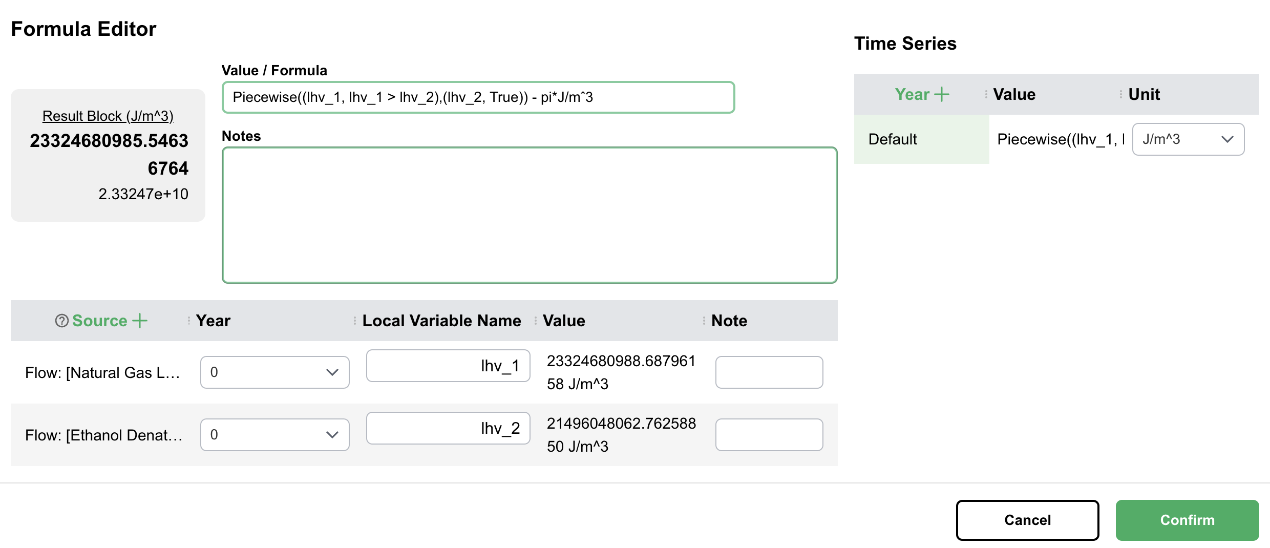
Formula Editor
This section supports defining parameters using formulas and variable references.
Using the Formula Editor
- Click into the Value / Formula cell to enter a formula
- The Result is shown in the Result Block on the left side
- Add any Notes to describe the formula in the notes box
- Any Errors will appear at the top of the formula editor
Acceptable Formulas
- Numeric values:
100.251 - Numeric formulas:
100 * 5 + 1 - Formulas with local parameters:
100 * parameter_1 - Numeric values accompanied by registered units:
pi * J/mˆ3(see figure)
Acceptable Formula Operations
The formula editor allows for most mathematical operations. These include the following functions:
| Function | Full Name | Example/Explanation |
|---|---|---|
max |
Maximum | max(3, 7, 2) → 7 |
ceil |
Ceiling | ceil(4.2) → 5 (rounds up to nearest integer) |
min |
Minimum | min(3, 7, 2) → 2 |
avg |
Average | avg(2, 4, 6) → 4 |
abs |
Absolute Value | abs(-5) → 5 |
log |
Natural Logarithm | log(e) → 1 (base e) |
exp |
Exponential | exp(2) → e² ≈ 7.389 |
sin |
Sine | sin(π/2) → 1 |
csc |
Cosecant | csc(x) = 1/sin(x) |
cos |
Cosine | cos(0) → 1 |
sec |
Secant | sec(x) = 1/cos(x) |
tan |
Tangent | tan(π/4) → 1 |
cot |
Cotangent | cot(x) = 1/tan(x) = cos(x)/sin(x) |
asin |
Arc Sine (Inverse Sine) | asin(1) → π/2 |
acsc |
Arc Cosecant | acsc(x) = asin(1/x) |
acos |
Arc Cosine (Inverse Cosine) | acos(1) → 0 |
asec |
Arc Secant | asec(x) = acos(1/x) |
atan |
Arc Tangent (Inverse Tangent) | atan(1) → π/4 |
acot |
Arc Cotangent | acot(1) → π/4 |
atan2 |
Two-Argument Arc Tangent | atan2(y, x) → angle in radians, accounts for quadrant |
sinh |
Hyperbolic Sine | sinh(x) = (eˣ - e⁻ˣ)/2 |
cosh |
Hyperbolic Cosine | cosh(x) = (eˣ + e⁻ˣ)/2 |
tanh |
Hyperbolic Tangent | tanh(x) = sinh(x)/cosh(x) |
coth |
Hyperbolic Cotangent | coth(x) = cosh(x)/sinh(x) |
sech |
Hyperbolic Secant | sech(x) = 1/cosh(x) |
asinh |
Inverse Hyperbolic Sine | asinh(x) = ln(x + √(x² + 1)) |
atanh |
Inverse Hyperbolic Tangent | atanh(0.5) ≈ 0.549 |
acoth |
Inverse Hyperbolic Cotangent | acoth(x) = atanh(1/x) |
asech |
Inverse Hyperbolic Secant | asech(x) = acosh(1/x) |
acsch |
Inverse Hyperbolic Cosecant | acsch(x) = asinh(1/x) |
acosh |
Inverse Hyperbolic Cosine | acosh(1) → 0 |
csch |
Hyperbolic Cosecant | csch(x) = 1/sinh(x) |
Piecewise((a₁, c₁), (a₂, c₂), ...) |
Piecewise Function | Piecewise((x, x>0), (-x, x<=0)) → returns x if positive, -x otherwise (absolute value) |
Note that nonlinear functions (e.g sin, cos, etc) do not support values with units.
Local Parameters Table
The local parameters table allows users to use other values from within PyGREET as variables within formulas.
Adding a Local Parameter
- Click the
+icon in the source column - Search for a parameter
- Parameters match based on text found within the search query
Parameter Format
Parameters take the form:
Note
A subsection is optional and may not be present.
Managing Local Parameters
When a local parameter is added, you can:
- View the value of the parameter
- Rename to provide a local meaninful name
- Select the time series year of the parameter
- Optionally add a note
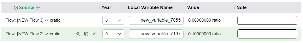
In addition, as shown in above figure, when hovering, you can:
- Remove the local parameter
- Click the magnifier icon to search the library for the parent object where the parameter was defined, using selective filtering, e.g.,
@Flow/NEW Flow 2 - Click the clipboard icon to copy the full path and locate where the parameter was declared in the parent object, e.g.,
Flow: [NEW Flow 2] -> cratio
Time Series Table
The time series table allows users to add time series data for a given parameter. When that parameter is used, it will use the time series data that is closest to the simulation year.
Example
If a parameter has data for 1999, 2010, and 2020, and the simulation year is 2006, it will use data from 2010.
Adding Time Series Data
- Click the
+icon next to the year column - Choose the desired year from the dropdown in the row added to the table
- Edit a given year by clicking on it in the time series data